Data Analysis

Load Packages

library(tidyverse)

── Attaching core tidyverse packages ──────────────────────── tidyverse 2.0.0 ──
✔ dplyr     1.1.4     ✔ readr     2.1.5
✔ forcats   1.0.0     ✔ stringr   1.5.1
✔ ggplot2   3.5.2     ✔ tibble    3.3.0
✔ lubridate 1.9.4     ✔ tidyr     1.3.1
✔ purrr     1.1.0     
── Conflicts ────────────────────────────────────────── tidyverse_conflicts() ──
✖ dplyr::filter() masks stats::filter()
✖ dplyr::lag()    masks stats::lag()
ℹ Use the conflicted package (<http://conflicted.r-lib.org/>) to force all conflicts to become errors

library(dplyr)
library(ggplot2)

Load Data

load("out/ai_investment_cleaned.RData")

Q1. AI total investment

p1 <- df_clean |> 
  group_by(Year) |>
  summarise(total_investment = sum(investment)) |>
  ggplot(aes(x = Year, y = total_investment)) +
  geom_line(size = 1) +
  # Add points
  geom_point(size = 2) +
  # Show all years
  scale_x_continuous(breaks = seq(min(df_clean$Year), 
                                  max(df_clean$Year), 
                                  by = 1)) + 
  labs(title = "AI total investment 2012-2025",
       x = "Year",
       y = "Sum of investments (USD millions)",
       caption = "Source: OEC") +
  theme_classic() 

Warning: Using `size` aesthetic for lines was deprecated in ggplot2 3.4.0.
ℹ Please use `linewidth` instead.

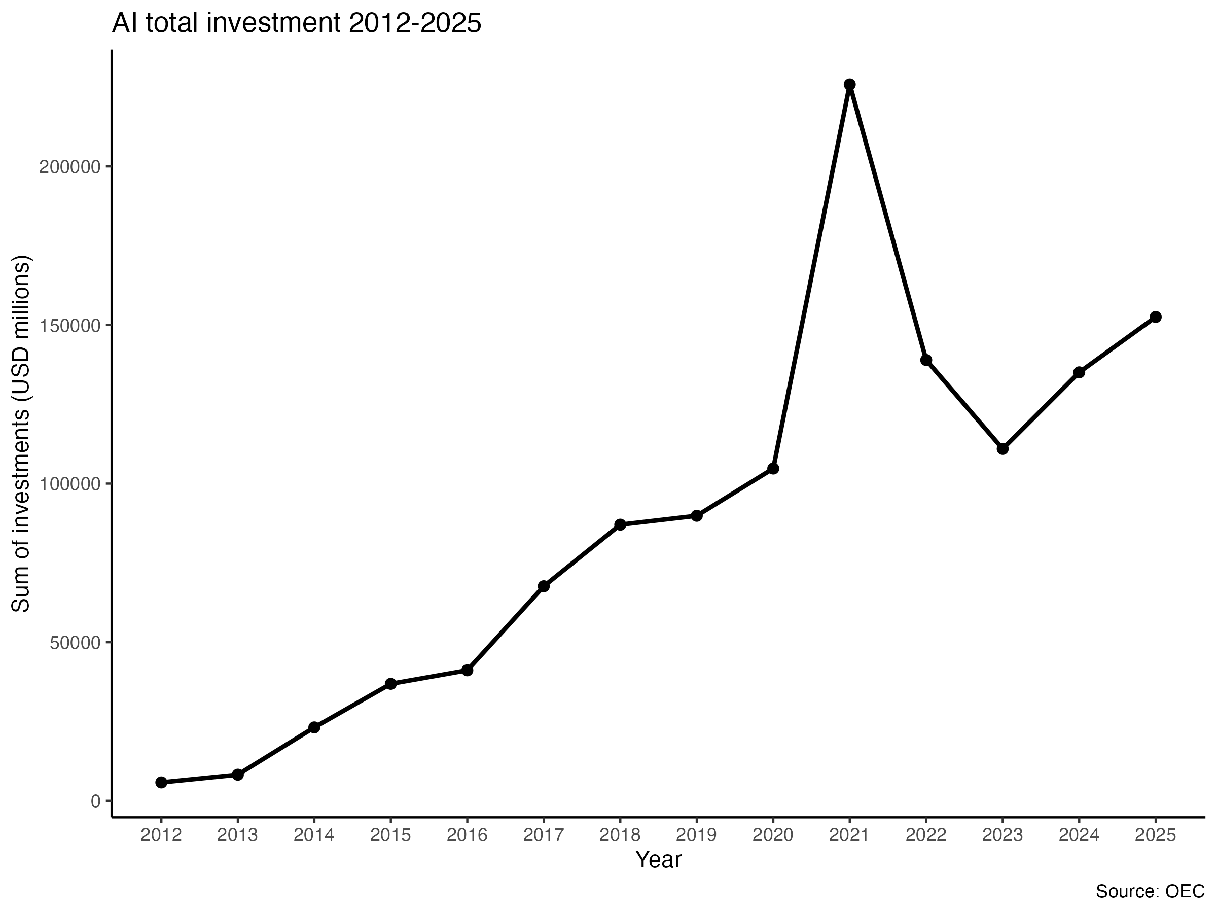
Global AI investment increased rapidly between 2020-2021.

# Save plot as PNG
ggsave("out/plot1.png", plot = p1, width = 8, height = 6, dpi = 300)

Q2. AI investment by industries in 2025

p2 <- df_clean |>
  filter(Year == max(Year)) |>
  arrange(-investment) |>
  ggplot(aes(x = fct_reorder(industry, investment), y = investment)) +
  geom_col(fill = "red") +
  labs(title = "AI investmen in different industry in 2025",
       x = "Industry",
       y = "Investment (USD millions)",
       caption = "Source: OEC") +
  theme_classic() +
  coord_flip() 

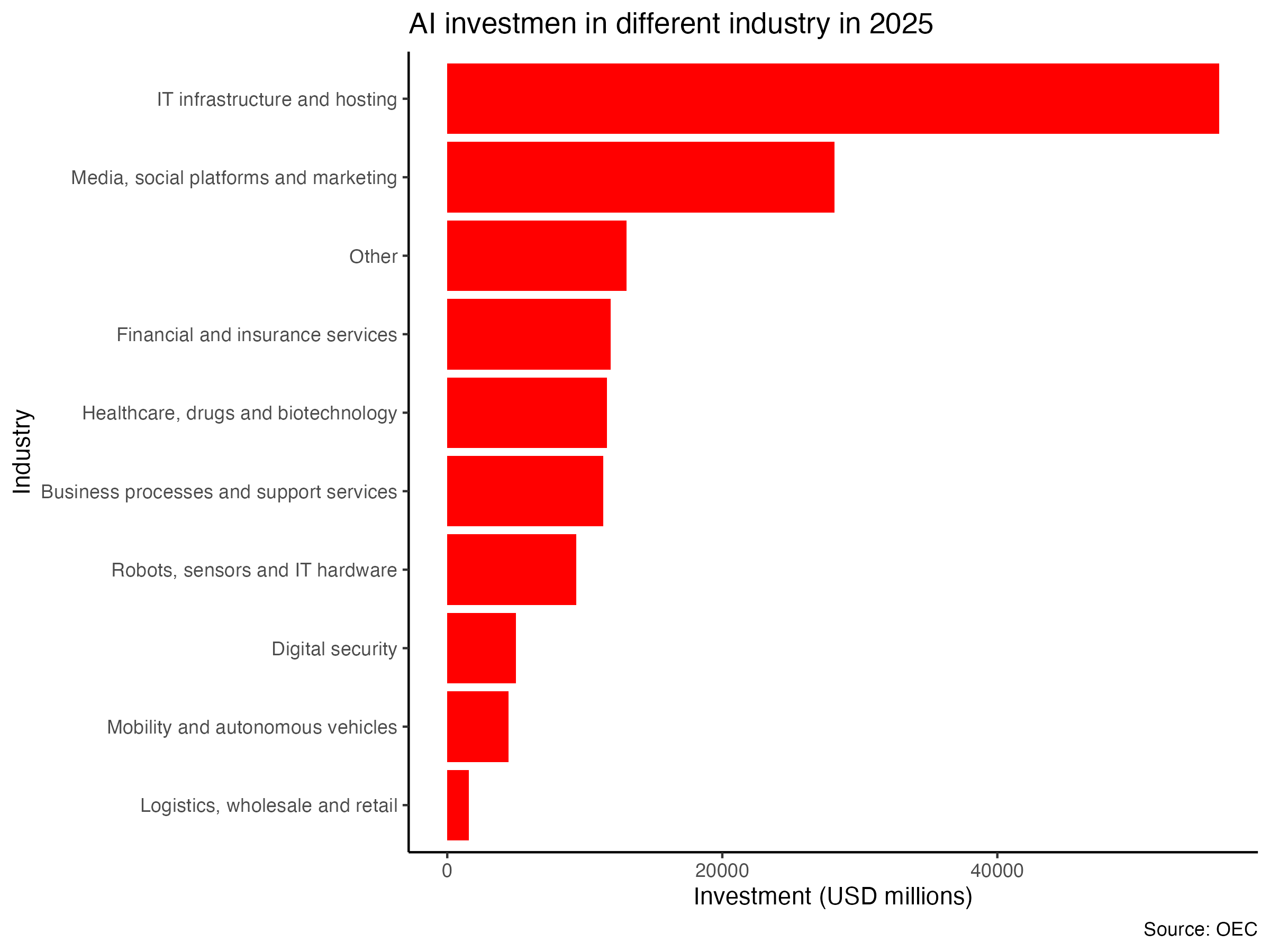
Most AI money still goes to business infrastructure like IT infrastructure and hosting.

# Save plot as PNG
ggsave("out/plot2.png", plot = p2, width = 8, height = 6, dpi = 300)

Q3. AI investment changes in different industries

p3 <- df_clean |>
  # 去掉 Other
  filter(industry != "Other") |>
 
  group_by(Year, industry) |>
  ggplot(aes(x = Year, y = investment, color = industry)) +
  geom_line() +
  labs(title = "AI investment in different industries from 2012 to 2025",
       x = "Year",
       y = "AI Investment (USD millions)",
       color = "Industry",
       caption = "Source: OEC") +
  theme_classic() +
  facet_wrap(~industry) +
  theme(legend.position = "none",
        strip.text = element_text(size = 7, face = "bold"))

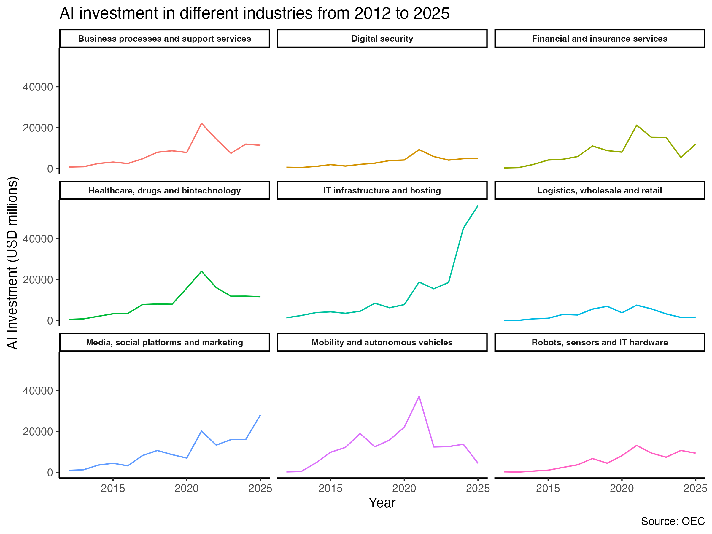
Different industries show distinct investment patterns. Most of money goes to IT and Media industry.

# Save plot as PNG
ggsave("out/plot3.png", plot = p3, width = 8, height = 6, dpi = 300)